ClimateDT-ROISelectionandDataAnalysis

Climate DT - ROI Selection and Monthly Analysis of Temperature/SWE correlation¶

Contents¶

Objective: This notebook has the aim to show how to request Climate DT data selecting a Region of Interest via HDA. The notebook shows also how to work with the obtained data.
Data Sources: https://destine.ecmwf.int/climate-change-adaptation-digital-twin-climate-dt/
Methods: The data request is performed using HDA REST API selecting a Region of Interest. The variables used in this notebook are the
- “2 metre temperature”, the temperature of air at 2m above the surface of land, sea or in-land waters.
- “snow depth”, the depth of snow in m of water equivalent.
  These two variable allow to check the correlation between the daily Temperature and the daily SWE (Snow Water Equivalent) Change (Accumulation/Melt). Daily snapshot temperature correlates with whether the snowpack tends to accumulate or melt.
```
When T < 0°C → snowfall tends to accumulate (SWE increases).
When T > 0°C → melt dominates (SWE decreases).
```
  The temperature controls the sign of SWE change.
Prerequisites:
- To search and access DEDL data a DestinE user account is needed
- To search and access DT data an upgraded access is needed.
Expected Output:
- 1 covjson files containing the requested data,
- 2 maps plot of the monthly mean of the 2 selcted variables,
- 1 scatter plot showing the correlation between the daily Temperature and the daily Snow Water Equivalent Accumulation/Melt.

Prerequisites¶

To run this tutorial, the appropriate access to the DestinE platform is needed:

To search and access DEDL data, a DestinE user account is required.
To access DT data, an upgraded access level is required.

Imports¶

pip install --user --quiet --upgrade destinelab

Note: you may need to restart the kernel to use updated packages.

import destinelab as deauth
import json
import requests
from urllib3.util.retry import Retry
import re
import sys
from requests.adapters import HTTPAdapter
from getpass import getpass
from tqdm import tqdm
import time
from datetime import datetime, timedelta

from IPython.display import JSON
import ipywidgets as widgets
from IPython.display import display, HTML
import xarray as xr
import matplotlib.pyplot as plt

Authentication¶

Authentication is required to access DestinE data.

Each DestinE user account provides access to the HDA API, which enables users to discover, query, and access the data products available to them on the platform. The level of data access depends on the user’s account type and granted permissions.

The destinelab package is used to perform the authentication.

DESP_USERNAME = input("Please input your DESP username: ")
DESP_PASSWORD = getpass("Please input your DESP password: ")

auth = deauth.AuthHandler(DESP_USERNAME, DESP_PASSWORD)
access_token = auth.get_token()
if access_token is not None:
    print("DEDL/DESP Access Token Obtained Successfully")
else:
    print("Failed to Obtain DEDL/DESP Access Token")

auth_headers = {"Authorization": f"Bearer {access_token}"}

Please input your DESP username:  eum-dedl-user
Please input your DESP password:  ········

DEDL/DESP Access Token Obtained Successfully

Configuration Constant¶

When accessing DestinE data through the HDA API, it is useful to define a small set of configuration constants upfront. These typically include:

The STAC API endpoint exposed by HDA
The region of interest
The collection name

HDA exposes data via a STAC‑compliant interface. While the collection name can be specified as a constant, it does not need to be known in advance, as available collections can be discovered dynamically using the HDA Discovery API searching for, e.g., Climate Change Adaptation Digital Twin.

HDA_STAC_ENDPOINT="https://hda.data.destination-earth.eu/stac/v2"
COLLECTION_ID="EO.ECMWF.DAT.D1.DT_CLIMATE.G1.SCENARIOMIP_SSP3-7.0_IFS-FESOM.R1"

#Central Alpine Box” (Switzerland–Northern Italy)
Alps_central={
      "type": "Polygon",
      "coordinates": [
        [
          [7.0, 45.7],
          [8.5, 45.7],
          [9.5, 46.3],
          [10.2, 47.0],
          [9.0, 47.7],
          [7.5, 47.6],
          [6.8, 46.8],
          [7.0, 45.7]
        ]
    ]
}

Utility Functions¶

Next, we define a few helper functions that will make it easier to gather the parameters needed to query the Climate DT collection.

# Fetch the collection metadata
def getParameters4collection(url,collection_id):
    response = requests.get(url)
    response.raise_for_status()
    collection = response.json()

    # Extract cube:variables
    cube_variables = collection.get("cube:variables", {})

    parsed_variables = {}

    for var_name, var_info in cube_variables.items():
        var_type = var_info.get("type")
        var_unit = var_info.get("unit")
        var_url = var_info.get("attrs").get("url")

        parsed_variables[var_name] = {
            "type": var_type,
            "unit": var_unit,
            "long_name": var_info.get("attrs").get("long_name"),
            "shortName": var_info.get("attrs").get("shortName"),
            "standard_name": var_info.get("attrs").get("standard_name"),
            "url": var_url,
            "parameter_ID": var_info.get("attrs").get("parameter_ID"),
            "product_type": var_info.get("attrs").get("product_type"),
            "levtype": var_info.get("attrs").get("levtype"),
            "levelist": var_info.get("attrs").get("levelist"),
            "time": var_info.get("attrs").get("time")
        }

    # Result: dictionary keyed by variable name
    #output = {collection_id: parsed_variables}
    #return output
    return parsed_variables

Search for snow depth and 2mt temperature data in a ROI¶

Our region of interest is the Central Alpine Box, covering Switzerland and Northern Italy, for which the polygon has been defined in the Configuration Constants section.

The variables available in the selected collection can be retrieved directly from its STAC metadata. Below, we list all parameters along with their relevant information.


# STAC collection URL
HDA_STAC_COLLECTION_ENDPOINT = HDA_STAC_ENDPOINT+'/collections/'+COLLECTION_ID

parameters=getParameters4collection(HDA_STAC_COLLECTION_ENDPOINT,COLLECTION_ID)

JSON(parameters)
#print(parameters)

From the list of available parameters, we select snow_depth and 2_metre_temperature at the surface level (levtype = sfc).

Using the metadata, we can extract the information required to formulate the HDA query and retrieve the desired product.

snow_depth = next(
    v for k, v in parameters.items()
    if "snow_depth" in k.lower() and v.get("levtype") == "sfc"
)
snow_depth

{'type': 'data',
 'unit': 'm of water equivalent',
 'long_name': 'Snow depth',
 'shortName': 'sd',
 'standard_name': 'Snow_depth',
 'url': 'https://codes.ecmwf.int/grib/param-db/141',
 'parameter_ID': '141',
 'product_type': 'forecast',
 'levtype': 'sfc',
 'levelist': '',
 'time': 'Hourly'}

t2 = next(
    v for k, v in parameters.items()
    if "2_metre_temperature" in k.lower() and v.get("levtype") == "sfc"
)
t2

{'type': 'data',
 'unit': 'K',
 'long_name': '2 metre temperature',
 'shortName': '2t',
 'standard_name': '2_metre_temperature',
 'url': 'https://codes.ecmwf.int/grib/param-db/167',
 'parameter_ID': '167',
 'product_type': 'forecast',
 'levtype': 'sfc',
 'levelist': '',
 'time': 'Hourly'}

snow depth is in meters of water equivalent, so it is effectively SWE (Snow Water Equivalent). WE use the HDA climate DT collection corresponding to the future projection (IFS-FESOM) - EO.ECMWF.DAT.D1.DT_CLIMATE.G1.SCENARIOMIP_SSP3-7.0_IFS-FESOM.R1

response = requests.post(HDA_STAC_ENDPOINT+"/search", headers=auth_headers, json={
 "collections": [COLLECTION_ID],
    "datetime": "2030-01-01T00:00:00Z/2030-01-30T23:00:00Z",
    "query":  {
    "ecmwf:resolution":{"eq": "high"},
    "ecmwf:levtype":{"eq": snow_depth["levtype"]},
    "ecmwf:time":{"eq": ["1200"]},
    "ecmwf:param":{"eq": [snow_depth["parameter_ID"],t2["parameter_ID"]]}
    },
    "intersects":Alps_central
})

if(response.status_code!= 200):
    (print(response.text))
response.raise_for_status()

product = response.json()["features"][0]
JSON(product)

Order and download snow depth and 2mt temperature data¶

The search results provide all the information required to place the order inside the retrieve link, including the order endpoint and the corresponding request body.

In the next cell, you can see how to extract these elements programmatically.


link = next((l for l in product.get('links', []) if l.get("rel") == "retrieve"), None)

if link:
    href = link.get("href")
    body = link.get("body")   # optional: depends on extension
    print("order endpoint:", href)
    print("order body:")
    print(json.dumps(body, indent=4))
else:
    print(f"No link with rel='{target_rel}' found")

order endpoint: https://hda.data.destination-earth.eu/stac/v2/collections/EO.ECMWF.DAT.D1.DT_CLIMATE.G1.SCENARIOMIP_SSP3-7.0_IFS-FESOM.R1/order
order body:
{
    "activity": "ScenarioMIP",
    "class": "d1",
    "dataset": "climate-dt",
    "date": "20300101/to/20300130",
    "experiment": "SSP3-7.0",
    "expver": "0001",
    "feature": {
        "shape": [
            [
                45.7,
                7.0
            ],
            [
                45.7,
                8.5
            ],
            [
                46.3,
                9.5
            ],
            [
                47.0,
                10.2
            ],
            [
                47.7,
                9.0
            ],
            [
                47.6,
                7.5
            ],
            [
                46.8,
                6.8
            ],
            [
                45.7,
                7.0
            ]
        ],
        "type": "polygon"
    },
    "generation": "1",
    "levtype": "sfc",
    "model": "IFS-FESOM",
    "param": [
        "141",
        "167"
    ],
    "realization": "1",
    "resolution": "high",
    "stream": "clte",
    "time": [
        "1200"
    ],
    "type": "fc"
}

Order¶

We can now submit the order and monitor its status until the product becomes available for download.

#Sometimes requests to polytope get timeouts, it is then convenient define a retry strategy
retry_strategy = Retry(
    total=10,  # Total number of retries
    status_forcelist=[500, 502, 503, 504, 400],  # List of 5xx status codes to retry on
    allowed_methods=["GET",'POST'],  # Methods to retry
    backoff_factor=1  # Wait time between retries (exponential backoff)
)

# Create an adapter with the retry strategy
adapter = HTTPAdapter(max_retries=retry_strategy)

# Create a session and mount the adapter
session = requests.Session()
session.mount("https://", adapter)


response = session.post(href, json=body, headers=auth_headers)


if response.status_code != 200:
    print(response.content)
response.raise_for_status()

ordered_item = response.json()

product_id = ordered_item["id"]
storage_tier = ordered_item["properties"].get("storage:tier", "online")
order_status = ordered_item["properties"].get("order:status", "unknown")
federation_backend = ordered_item["properties"].get("federation:backends", [None])[0]

print(f"Order status: {order_status}")   


#timeout and step for polling (sec)
TIMEOUT = 300
STEP = 1
ONLINE_STATUS = "online"

self_url = f"{HDA_STAC_ENDPOINT}/collections/{COLLECTION_ID}/items/{product_id}"
item = {}

for i in range(0, TIMEOUT, STEP):
    print(f"Polling {i + 1}/{TIMEOUT // STEP}")

    response = session.get(self_url, headers=auth_headers)
    if response.status_code != 200:
        print(response.content)
    response.raise_for_status()
    item = response.json()

    storage_tier = item["properties"].get("storage:tier", ONLINE_STATUS)

    if storage_tier == ONLINE_STATUS:
        download_url = item["assets"]["downloadLink"]["href"]
        print("Product is ready to be downloaded.")
        print(f"Download URL: {download_url}")
        break

    time.sleep(STEP)
else:
    order_status = item["properties"].get("order:status", "unknown")
    print(f"We could not download the product after {TIMEOUT // STEP} tries. Current order status is {order_status}")

Order status: ordered
Polling 1/300
Polling 2/300
Polling 3/300
Polling 4/300
Product is ready to be downloaded.
Download URL: https://hda-download.leonardo.data.destination-earth.eu/data/dedt_mn5/EO.ECMWF.DAT.D1.DT_CLIMATE.G1.SCENARIOMIP_SSP3-7.0_IFS-FESOM.R1/89f67081-64fb-4cd0-aced-05ea417e81dd/downloadLink

Download¶

The download url can then be used to download the product

response = session.get(download_url, stream=True, headers=auth_headers)
response.raise_for_status()

content_disposition = response.headers.get('Content-Disposition')
total_size = int(response.headers.get("content-length", 0))
if content_disposition:
    ext = re.search(r'\.(\w+)', content_disposition).group(0)
    filename = 'swe_2t_jan_2030'+ext
else:
    filename = os.path.basename(product_id)

# Open a local file in binary write mode and write the content
print(f"downloading {filename}")

with tqdm(total=total_size, unit="B", unit_scale=True) as progress_bar:
    with open(filename, 'wb') as f:
        for data in response.iter_content(1024):
            progress_bar.update(len(data))
            f.write(data)

downloading swe_2t_jan_2030.covjson

2.40MB [00:00, 11.0MB/s]

Load and Visualize data using Earthkit¶

In this section, we load the downloaded dataset using Earthkit, which provides a simple and efficient interface for this data.

After loading the data, we visualize the selected variable over our region of interest to quickly inspect its spatial distribution and confirm that the product has been retrieved correctly.

pip install --quiet --user covjsonkit

Note: you may need to restart the kernel to use updated packages.

import earthkit.data
data = earthkit.data.from_source("file", filename)

We can now transform data in xarray

data.to_xarray()

In the cell below:

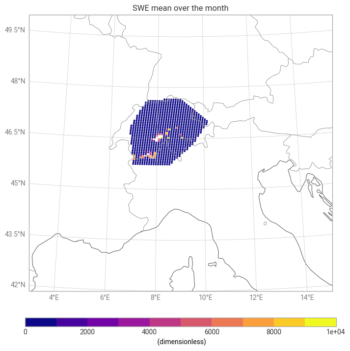
Unit conversion: Convert snow_depth [m] → [mm] by multiplying by 1000.
*Mean": Compute the mean value at the same hour for all days within the selected month.
Visualization: Plot the resulting monthly mean snow-depth map over the ROI.

import earthkit.plots
swe_2t_xr = data.to_xarray()
swe_2t_xr ['sd']= swe_2t_xr['sd'] * 1000.0  # m -> mm


mean_swe = swe_2t_xr['sd'].mean(dim="datetimes")   # average over time

print(mean_swe.min().item(), mean_swe.max().item())

chart_sd = earthkit.plots.Map(domain=[3, 15, 42, 50])
chart_sd.point_cloud(mean_swe, x="longitude", y="latitude")

chart_sd.coastlines()
chart_sd.borders()
chart_sd.gridlines()

chart_sd.title("SWE mean over the month")

chart_sd.legend()

chart_sd.show()

In the cell below:

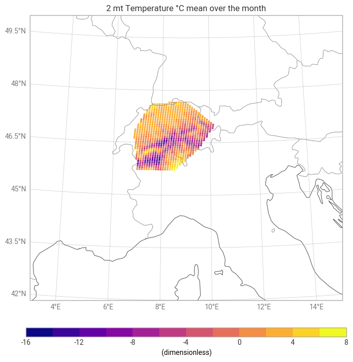
Unit conversion: Convert temperature [K] → [°C]
*Mean": Compute the mean value at the same hour for all days within the selected month.
Visualization: Plot the resulting monthly mean snow-depth map over the ROI.

swe_2t_xr['2t']= swe_2t_xr['2t'] - 273.15  # K -> °C
chart_2t = earthkit.plots.Map(domain=[3, 15, 42, 50])

mean_2t=swe_2t_xr['2t'].mean("datetimes")

print(mean_2t.min().item(), mean_2t.max().item())

chart_2t.point_cloud(mean_2t, x="longitude", y="latitude")

chart_2t.coastlines()
chart_2t.borders()
chart_2t.gridlines()

chart_2t.title("2 mt Temperature °C mean over the month")

chart_2t.legend()

chart_2t.show()

-14.693413035074848 6.871611531575543

#lon = t2['longitude'].values
#lat = t2['latitude'].values

Inspect Time Coverage and Data Ranges¶

This cell provides a quick diagnostic summary of the loaded dataset.

It prints the time coverage (all available timestamps) and reports the value ranges for the key variables—temperature and snow depth.

These checks help confirm that the dataset has been loaded correctly, the temporal dimension matches expectations, and the physical variables fall within a reasonable range before proceeding with further analysis.

print("Time coverage:", swe_2t_xr.datetimes.values)
print("Temperature range:", float(swe_2t_xr["2t"].min()),
      float(swe_2t_xr["2t"].max()))
print("Snow depth range:", float(swe_2t_xr["sd"].min()),
      float(swe_2t_xr["sd"].max()))

Time coverage: ['2030-01-01 12:00:00Z' '2030-01-02 12:00:00Z' '2030-01-03 12:00:00Z'
 '2030-01-04 12:00:00Z' '2030-01-05 12:00:00Z' '2030-01-06 12:00:00Z'
 '2030-01-07 12:00:00Z' '2030-01-08 12:00:00Z' '2030-01-09 12:00:00Z'
 '2030-01-10 12:00:00Z' '2030-01-11 12:00:00Z' '2030-01-12 12:00:00Z'
 '2030-01-13 12:00:00Z' '2030-01-14 12:00:00Z' '2030-01-15 12:00:00Z'
 '2030-01-16 12:00:00Z' '2030-01-17 12:00:00Z' '2030-01-18 12:00:00Z'
 '2030-01-19 12:00:00Z' '2030-01-20 12:00:00Z' '2030-01-21 12:00:00Z'
 '2030-01-22 12:00:00Z' '2030-01-23 12:00:00Z' '2030-01-24 12:00:00Z'
 '2030-01-25 12:00:00Z' '2030-01-26 12:00:00Z' '2030-01-27 12:00:00Z'
 '2030-01-28 12:00:00Z' '2030-01-29 12:00:00Z' '2030-01-30 12:00:00Z']
Temperature range: -26.23211517333982 11.962083435058616
Snow depth range: 0.0 10000.0

Compute daily SWE change (ΔSWE)¶

Compute daily SWE change: ΔSWE=SWE(t)−SWE(t−1)

Positive ΔSWE = snowfall accumulation
Negative ΔSWE = melt / compaction

Delta_SWE = swe_2t_xr["sd"].diff('datetimes')
Delta_SWE.attrs['units'] = 'mm/day'

T_for_scatter = swe_2t_xr["2t"].isel(datetimes=slice(1, None))
SWE_for_scatter = swe_2t_xr["sd"].isel(datetimes=slice(1, None))
Delta_for_scatter = Delta_SWE

print("Days in month:", swe_2t_xr["2t"].datetimes.size)
print("Scatter samples:", T_for_scatter.datetimes.size)

Days in month: 30
Scatter samples: 29

import numpy as np
# Build a DataFrame for statistics
import warnings
warnings.filterwarnings('ignore')

df = xr.merge([T_for_scatter, Delta_for_scatter]).to_dataframe().dropna()
plt.figure(figsize=(7,5))
plt.scatter(df['2t'], df['sd'], color='tab:red', alpha=0.8, label='Daily points')
plt.axhline(0, color='gray', lw=1)
plt.xlabel('Daily T (°C)')
plt.ylabel('ΔSWE (mm/day)')
plt.title(f'Temperature vs ΔSWE')
plt.legend()
plt.tight_layout()
plt.show()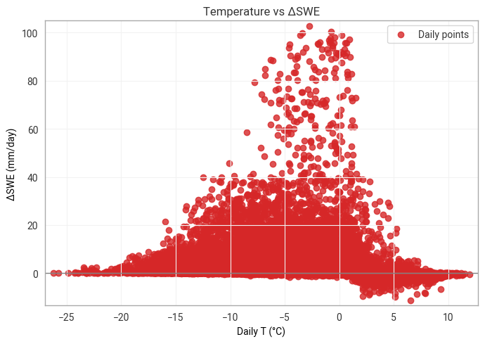

Summary¶

Throughout this notebook, we demonstrated how to query and download temperature and snow‑depth data from the HDA within a defined region of interest for a month at a certain hour.

We used Earthkit to load and visualize data. We inspected the dataset’s spatial and temporal coverage, performed unit conversions, and computed a monthly mean over the ROI.

Finally, by examining the relationship between temperature and snow depth, we visualized their correlation highlighting how temperature fluctuations relate to snowpack variability.

Overall, the workflow showcased a complete end‑to‑end approach—from data discovery and retrieval to visualization and statistical analysis—illustrating how HDA and Earthkit can be combined to efficiently explore climate variables over a specific region.

Resources and references¶

References:

Credit:

Earthkit packages used in this context are provided by the European Centre for Medium-Range Weather Forecasts (ECMWF).