ExtremeDT Weather Data Cubes - DEDL Notebook Gallery

Data Cube populated with data obtained from Weather and Geophysical Extremes Digital Twin (DT) - ExtremeDT¶

This notebook covers:

find available data cubes and their urls
upload data cube
plot map for desired area, time and variable
plot time series chart for selected variable in specifc time for specific location
create interactive dashboard using xcube - xviewer

Prepre your environment¶

import xarray as xr
import numpy as np
import matplotlib.pyplot as plt
import dask
import requests

Connect with Extreme DT data cube¶

The data cube provides data:

Four variables
- 2t - Air temperature at 2 meters above grond [K]
- 2d - Dew point temperature at 2 meters above grond [K]
- sp - Surface pressure [Pa]
Forecast from 10.04.2024 + 96 hours
Hourly step
World

Select proper data cube¶

Data cubes on s3 bucket are stored under URL https://s3.central.data.destination-earth.eu/swift/v1/dedl_datacube.
Data cubes are stored in two directories:

ExtremeDT - the newest one
archive - from prievous days

File nameing convention:
dt_extreme_YYYYMMDD.zarr/
YYYYMMDD - is the date when forecast starts (step 0)

Results
After exectution of code below, the list of urls linked to available cubes will be printed.

# URL to s3 where  ExtremeDT data cubes are stored
datacube_url = 'https://s3.central.data.destination-earth.eu/swift/v1/dedl_datacube'
response = requests.get(datacube_url)

if response.status_code == 200:
    lines = response.text.splitlines()
    zarr_items = [line for line in lines if line.endswith(".zarr") or line.endswith(".zarr/")]
    if zarr_items:
        for item in zarr_items:
            print(item)
            new_url = f"{datacube_url}/{item}"
            print("New URL:", new_url)
    else:
        print("No .zarr files or directories found.")
else:
    print("Failed to fetch contents. Status code:", response.status_code)

ExtremeDT/dt_extreme_20240410.zarr/
New URL: https://s3.central.data.destination-earth.eu/swift/v1/dedl_datacube/ExtremeDT/dt_extreme_20240410.zarr/
archive/dt_extreme_20240409.zarr/
New URL: https://s3.central.data.destination-earth.eu/swift/v1/dedl_datacube/archive/dt_extreme_20240409.zarr/

Get info about the newset data cube.

# Paste into url variable link to the newest data cube
url = 'https://s3.central.data.destination-earth.eu/swift/v1/dedl_datacube/ExtremeDT/dt_extreme_20240410.zarr/'

Let’s make some test¶

Area of interest¶

Upload data for selected area and verify what variables are provided. In this case uplaod data for Africa. List of available variables should be returend.

africa_bbox = [-20,     # West
                -40,    # South
                60,     # East
                40]     #North

africa_dt = xr.open_zarr(url).sel(lon=slice(africa_bbox[0], 
                                            africa_bbox[2]), 
                                lat=slice(africa_bbox[3], 
                                            africa_bbox[1]),
                                                         )

list(africa_dt.keys())

['2d', '2t', 'sp']

Plot map of air temperature for Africa.

lon = africa_dt['lon']
lat = africa_dt['lat']
temperature = africa_dt['2t'][0, 0] - 273.15 # Conversion to Celcius degrees

plt.figure(figsize=(10, 6))
plt.pcolormesh(lon, lat, temperature, cmap='coolwarm')
plt.colorbar(label='Temperature (°C)')
plt.title('Temperature Map')
plt.xlabel('Longitude')
plt.ylabel('Latitude')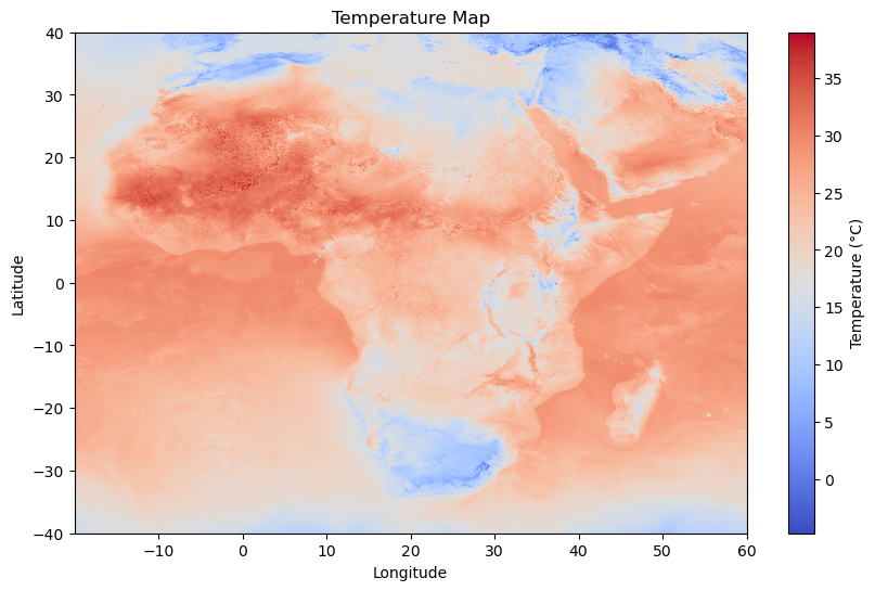

Get data for specific time range¶

Get data from 10st of April to 11th of April.

africa_bbox = [-20,     # West
                -40,    # South
                60,     # East
                40]     #North

africa_dt = xr.open_zarr(url).sel(lon=slice(africa_bbox[0], 
                                            africa_bbox[2]), 
                                lat=slice(africa_bbox[3], 
                                            africa_bbox[1]),
                                time=slice('20240410T000000', '20240411T000000')
                                                         )

print(africa_dt.time)

<xarray.DataArray 'time' (time: 25)>
array(['2024-04-10T00:00:00.000000000', '2024-04-10T01:00:00.000000000',
       '2024-04-10T02:00:00.000000000', '2024-04-10T03:00:00.000000000',
       '2024-04-10T04:00:00.000000000', '2024-04-10T05:00:00.000000000',
       '2024-04-10T06:00:00.000000000', '2024-04-10T07:00:00.000000000',
       '2024-04-10T08:00:00.000000000', '2024-04-10T09:00:00.000000000',
       '2024-04-10T10:00:00.000000000', '2024-04-10T11:00:00.000000000',
       '2024-04-10T12:00:00.000000000', '2024-04-10T13:00:00.000000000',
       '2024-04-10T14:00:00.000000000', '2024-04-10T15:00:00.000000000',
       '2024-04-10T16:00:00.000000000', '2024-04-10T17:00:00.000000000',
       '2024-04-10T18:00:00.000000000', '2024-04-10T19:00:00.000000000',
       '2024-04-10T20:00:00.000000000', '2024-04-10T21:00:00.000000000',
       '2024-04-10T22:00:00.000000000', '2024-04-10T23:00:00.000000000',
       '2024-04-11T00:00:00.000000000'], dtype='datetime64[ns]')
Coordinates:
  * time     (time) datetime64[ns] 2024-04-10 2024-04-10T01:00:00 ... 2024-04-11
Attributes:
    axis:           T
    standard_name:  time

Obtain data for specific variable and time¶

Obtain surface pressure data from 10th of April to 11th of April.

africa_bbox = [-20,     # West
                -40,    # South
                60,     # East
                40]     #North

africa_dt = xr.open_zarr(url)['sp'].sel(lon=slice(africa_bbox[0], 
                                            africa_bbox[2]), 
                                lat=slice(africa_bbox[3], 
                                            africa_bbox[1]),
                                time=slice('20240410T000000', '20240411T000000')
                                                         )

print(africa_dt.var)

<bound method DataArrayAggregations.var of <xarray.DataArray 'sp' (time: 25, lat: 2276, lon: 2279)>
dask.array<getitem, shape=(25, 2276, 2279), dtype=float32, chunksize=(25, 417, 837), chunktype=numpy.ndarray>
Coordinates:
  * lat      (lat) float64 39.99 39.95 39.92 39.88 ... -39.92 -39.95 -39.99
  * lon      (lon) float64 -19.97 -19.94 -19.9 -19.87 ... 59.92 59.95 59.99
  * time     (time) datetime64[ns] 2024-04-10 2024-04-10T01:00:00 ... 2024-04-11
Attributes:
    CDI_grid_num_LPE:  2560
    CDI_grid_type:     gaussian
    long_name:         Surface pressure
    param:             0.3.0
    standard_name:     surface_air_pressure
    units:             Pa>

Plot map of surface pressure over Africa.

lon = africa_dt['lon']
lat = africa_dt['lat']
temperature = africa_dt[0] / 100    # Conversion to hectoPascals

plt.figure(figsize=(10, 6))
plt.pcolormesh(lon, lat, temperature, cmap='viridis')
plt.colorbar(label='Surface Pressure (hPa)')
plt.title('Surface pressure Map')
plt.xlabel('Longitude')
plt.ylabel('Latitude')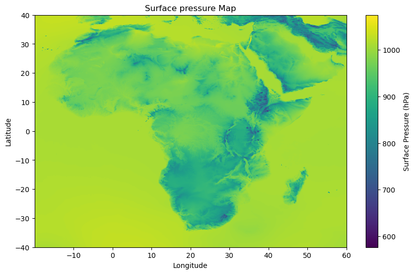

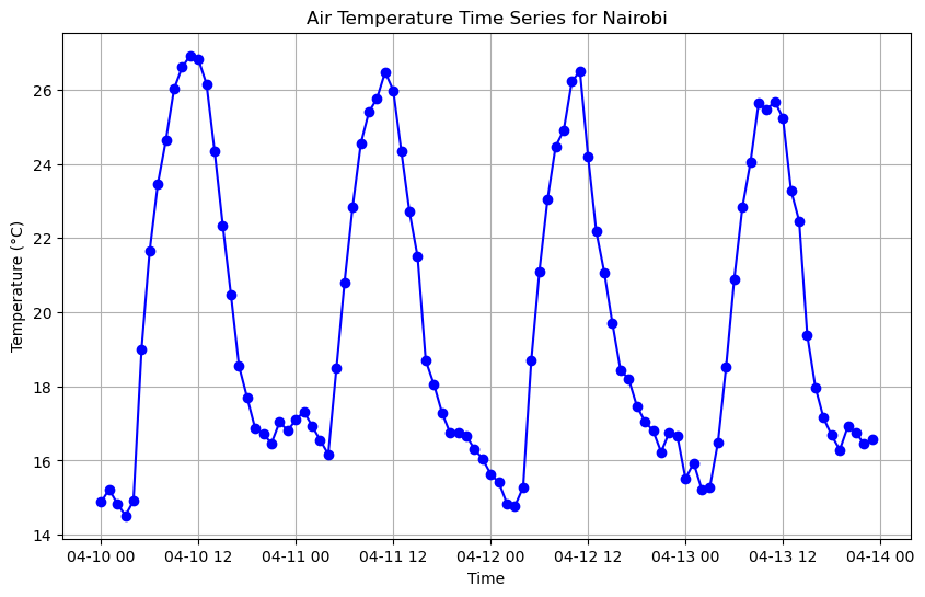
Time series¶

Verify if it is possible to create time series chart (for 96 hours) from DT output - air temperature over Nairobi.

africa_bbox = [-20,     # West
                -40,    # South
                60,     # East
                40]     #North

africa_dt = xr.open_zarr(url).sel(lon=slice(africa_bbox[0], 
                                            africa_bbox[2]), 
                                lat=slice(africa_bbox[3], 
                                            africa_bbox[1]),
                                )

Create a chart.

# Define Nairobi coordinates
nairobi_lat = -1.286389
nairobi_lon = 36.817223

lat = africa_dt['lat']
lon = africa_dt['lon']
nearest_lat_idx = np.abs(lat - nairobi_lat).argmin()
nearest_lon_idx = np.abs(lon - nairobi_lon).argmin()

temperature_nairobi = africa_dt['2t'][:, :, nearest_lat_idx, nearest_lon_idx] - 273.15
time_values = africa_dt.time.values

plt.figure(figsize=(10, 6))
plt.plot(time_values, temperature_nairobi, marker='o', color='b')
plt.title('Air Temperature Time Series for Nairobi')
plt.xlabel('Time')
plt.ylabel('Temperature (°C)')
plt.grid(True)
plt.show()